Average-flow estimate
Using propellant mass, burn time, throat area, and characteristic velocity gave an estimated 742 psi chamber pressure.
Rowan University / CFD / Spring 2025
Resolving the flow.
Understanding the thrust.
A team study of supersonic flow through the AeroTech J350W rocket nozzle, using ANSYS Fluent to connect nozzle geometry, mesh quality, solver behavior, and propulsion performance.
01 / The project
The objective was to model expansion through a solid rocket motor nozzle, resolve the supersonic plume, and estimate thrust from the nozzle-exit flow properties.
The AeroTech J350W provided a commercial motor with reference thrust data for comparison. Our team used a simplified axisymmetric model to explore how the domain, mesh, boundary conditions, and numerical methods affected the result.
Zach Pedrick, James Lee, and Glen Vosgerichian · Rowan University · Spring 2025.
This page presents our shared team study. The report does not assign individual responsibilities, so the work is credited collectively.
02 / Geometry & domain
The initial domain included the internal combustion chamber and a large surrounding region. Early runs showed that this added computational cost without improving the flow resolution near the exit.
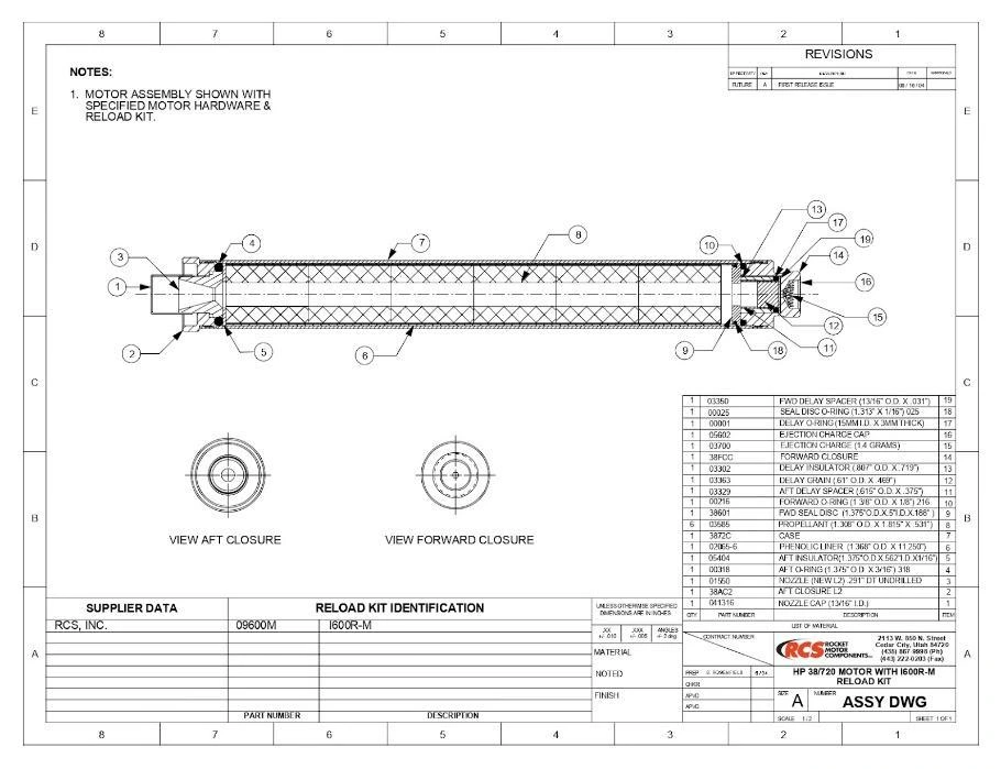
The team removed the combustion chamber and applied a pressure inlet directly at the nozzle entrance. A half-section, treated as axisymmetric, retained the rotational geometry while reducing the computational problem to two dimensions.
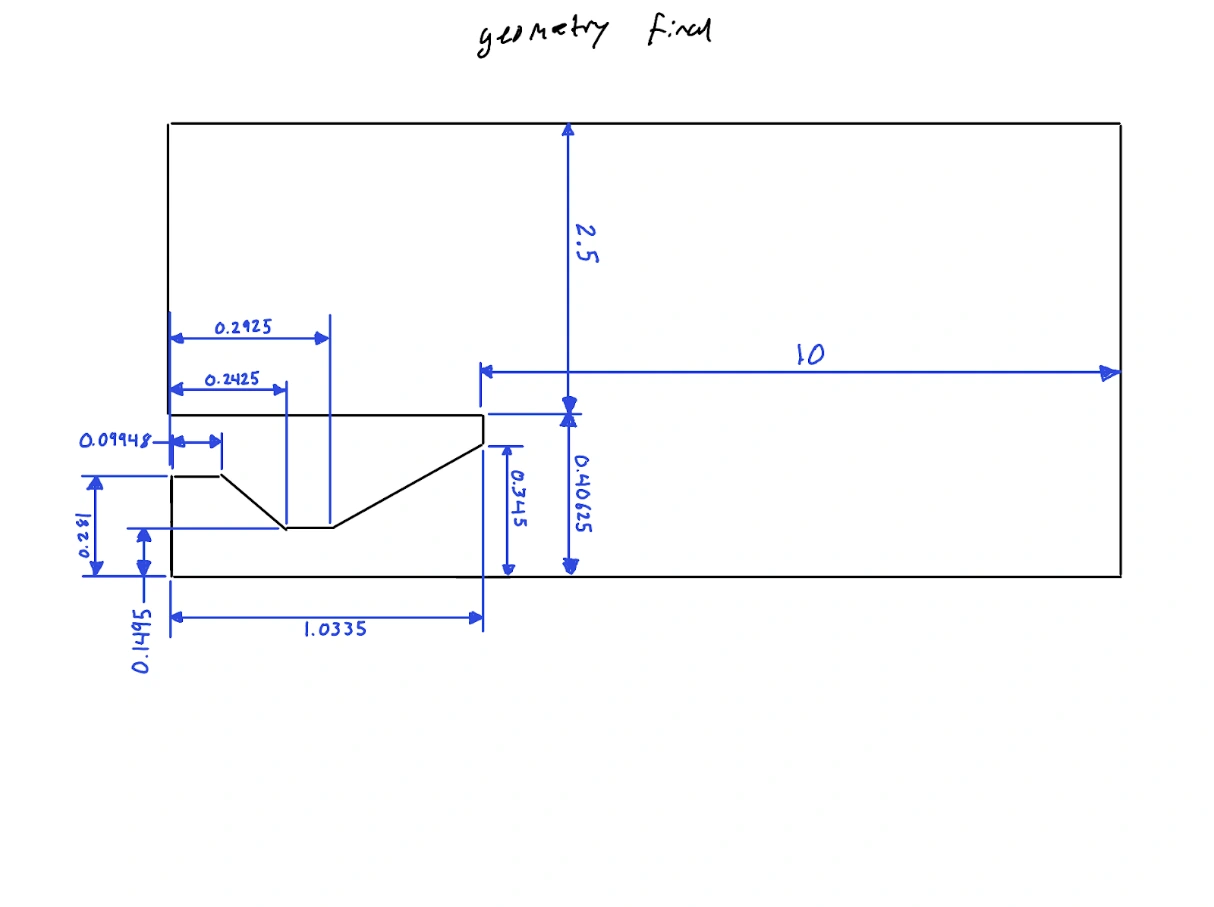
The surrounding domain was reduced while retaining space for plume expansion. A region above the nozzle allowed the exhaust’s interaction with ambient air to appear in the solution.
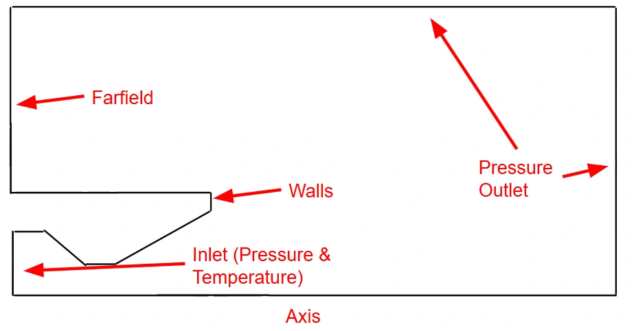
The boundary layout distinguishes the inlet, solid walls, symmetry axis, farfield region, and pressure outlets. Combustion itself was outside the model: inlet conditions represented its effect on the nozzle flow.
Read the original explanation · PDF p. 5 ↗03 / Grid development
The team documented 17 mesh versions, adjusting element type, edge sizing, and biasing. Critical regions included the throat, nozzle exit, and expanding plume. The final approach favored quadrilateral elements and a structured multizone mesh.
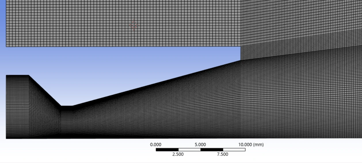
Quality checks included aspect ratio, skewness, and orthogonal quality. Local throat sizing reached 0.1 mm in the study, while reducing the external domain helped control the overall element count.
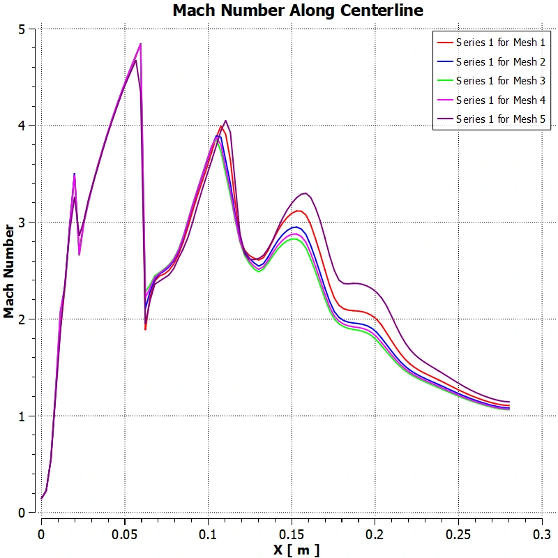
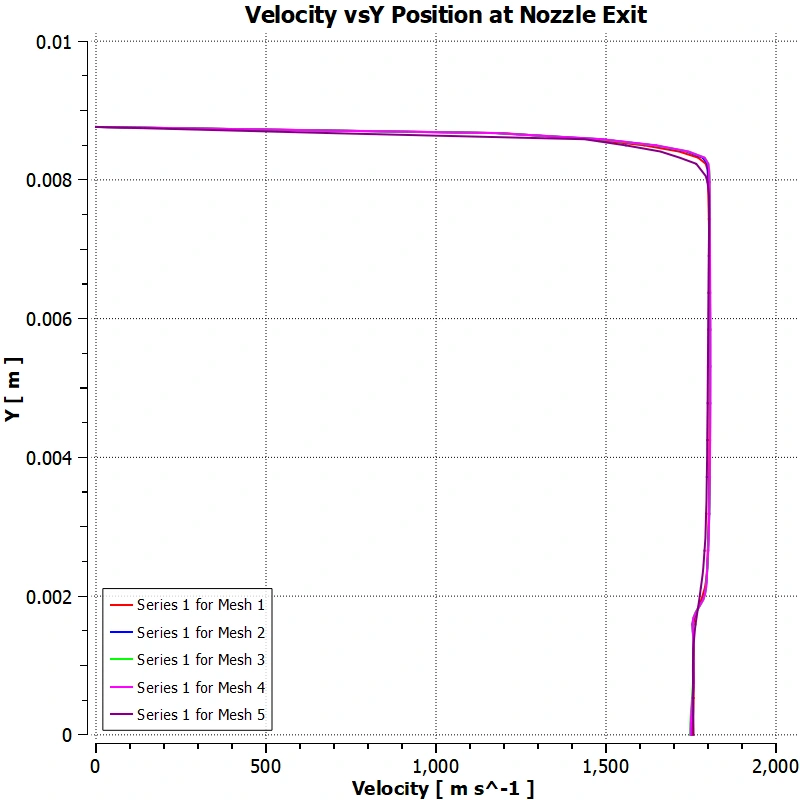
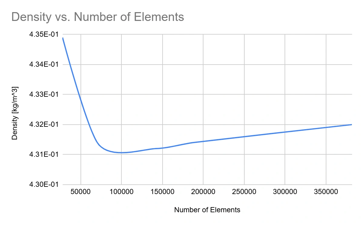
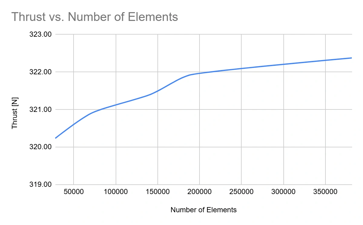
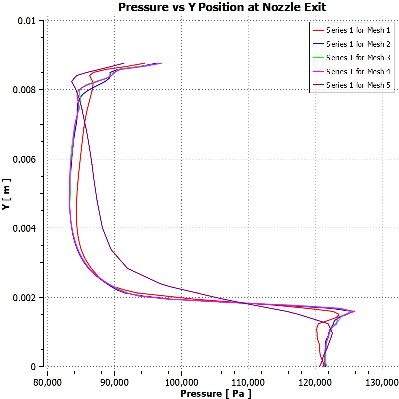
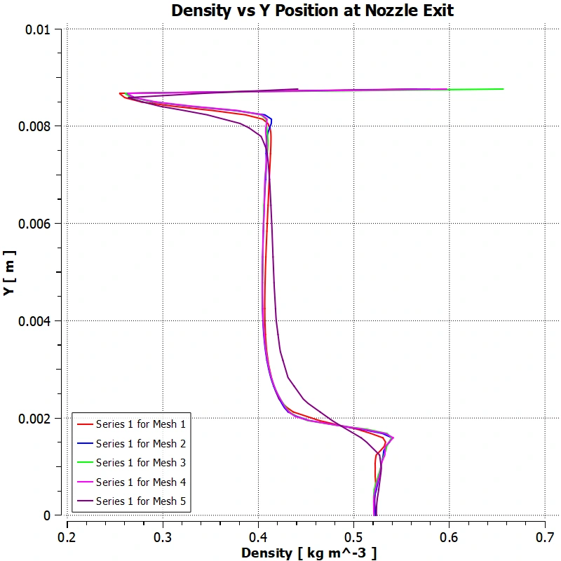
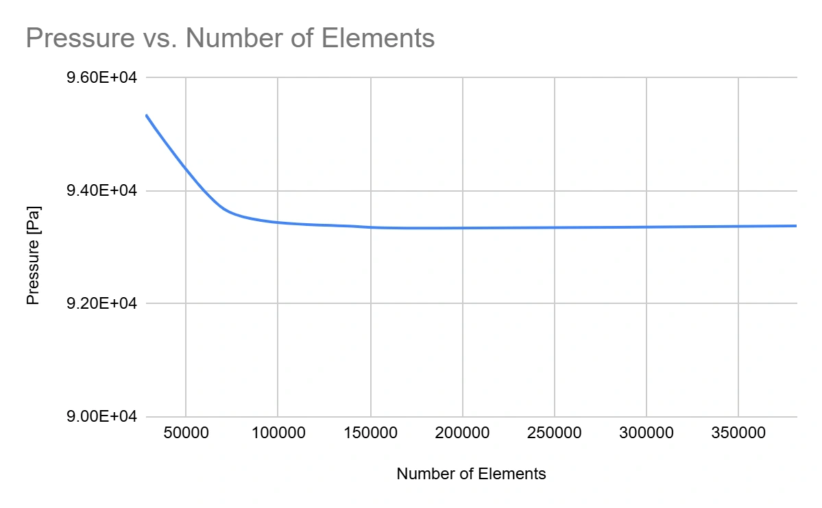
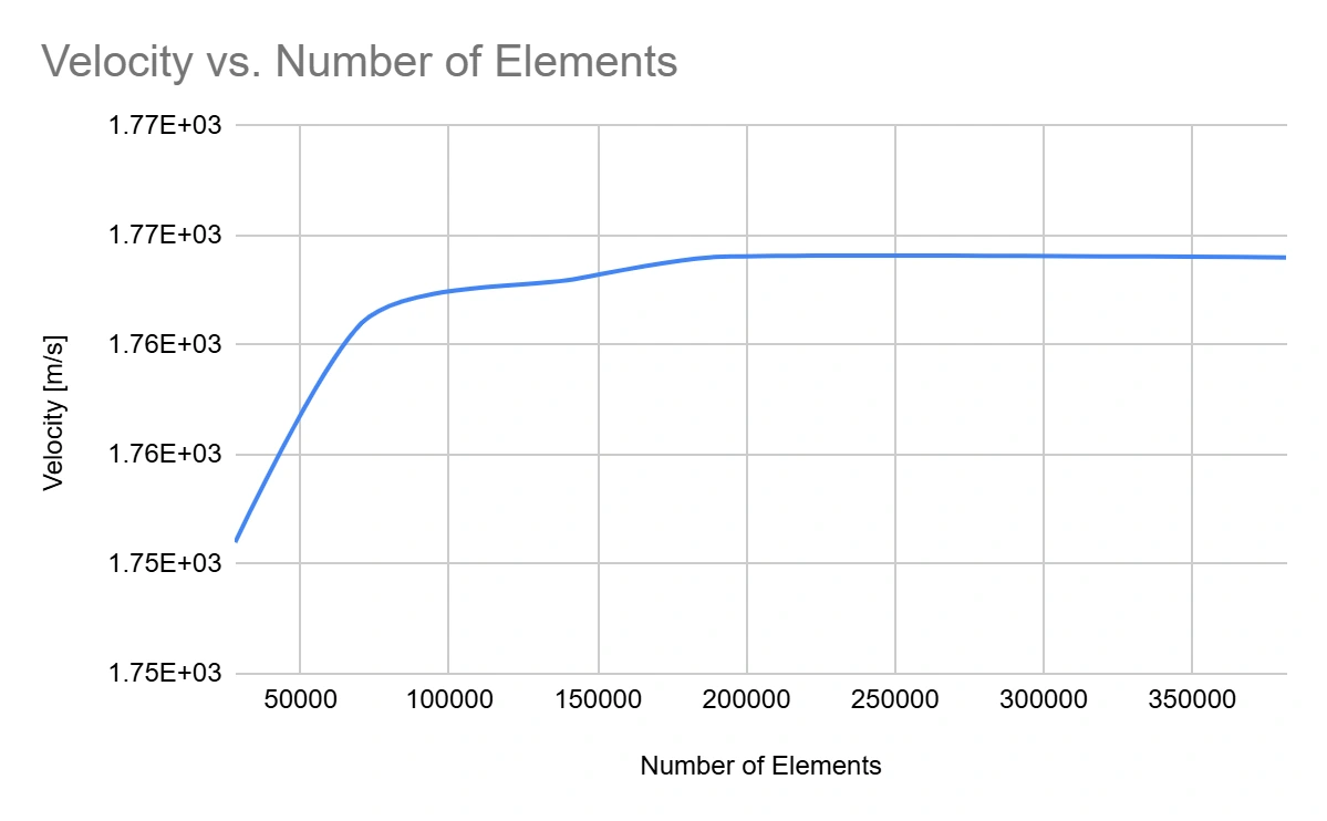
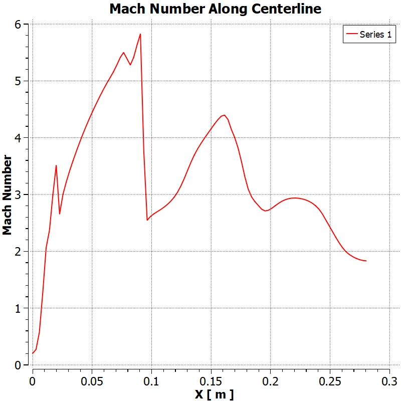
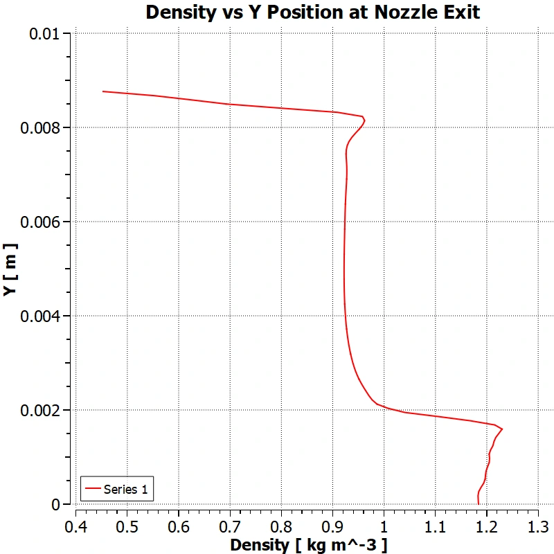
The grid study examined Mach number along the centerline and velocity, pressure, and density at the nozzle exit. Averaged exit quantities and thrust provided another view of how the solution changed with element count.
| Case | Elements | Aspect ratio | Skewness | Initial outcome |
|---|---|---|---|---|
| 1 | 70,502 | 1.7797 | 0.0559 | Converged |
| 2 | 141,771 | 1.9861 | 0.0626 | Did not converge |
| 3 | 381,880 | 2.7808 | 0.0752 | Did not converge |
| 4 | 187,433 | 2.0555 | 0.0652 | Did not converge |
| 5 | 27,980 | 1.3557 | 0.0296 | Converged |
Mesh 2, identified as iteration 13, was selected at approximately 142,000 elements. Its continuity residual had not converged during the grid-study stage; the team retained it and continued changing solver settings. The final residual history appears in the solver section below.
The grid-study plots suggested diminishing changes in several exit quantities. However, unresolved continuity in the selected grid limits how strongly that stage alone establishes mesh independence.
04 / Boundary conditions
The inlet required chamber pressure and temperature representative of motor operation. The report used OpenMotor’s White Lightning propellant data to support estimates, then explored three methods for chamber pressure.
Using propellant mass, burn time, throat area, and characteristic velocity gave an estimated 742 psi chamber pressure.
A relation using grain burn area and propellant parameters gave 530 psi. Low calculated thrust prompted further investigation.
The team used published J350W thrust data with a nozzle-thrust relation to infer pressure. The final inlet used an initial value of 1,738 psi.
The simulation used fixed inlet conditions and ambient outlet conditions, representing a steady operating point rather than an entire burn.
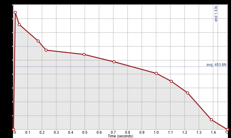
Reference thrust helped establish the inlet pressure and also supplied the peak value used for the final comparison. Agreement with that peak is useful as a consistency check, but it is not a fully independent validation of the model.
05 / Numerical development
The team first tried a pressure-based solver, then moved to a density-based solver for the highly compressible flow. Although the latter improved the flow representation, convergence and computational cost remained difficult.
The final setup returned to a pressure-based coupled solver with realizable k–epsilon turbulence modeling, the energy equation enabled, and second-order upwind discretization. Spalart–Allmaras and the Reynolds Stress Model were also tested; the report describes tradeoffs in shock resolution, speed, and stability.
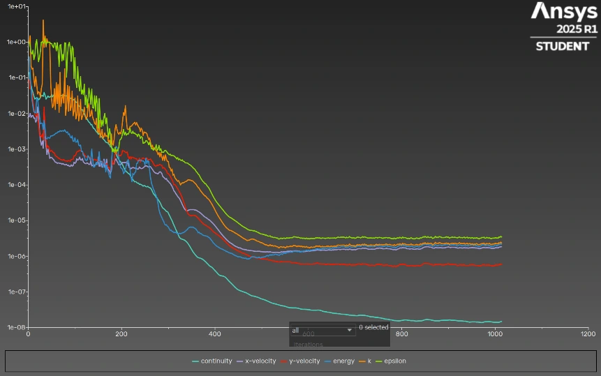
The final report describes improved residual behavior and resolved shock diamonds. The history above records that behavior directly; the report does not provide a numerical residual acceptance threshold or a separate mass-balance check.
Read the original explanation · PDF p. 12 ↗06 / Flow & performance
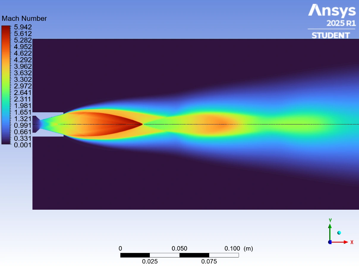
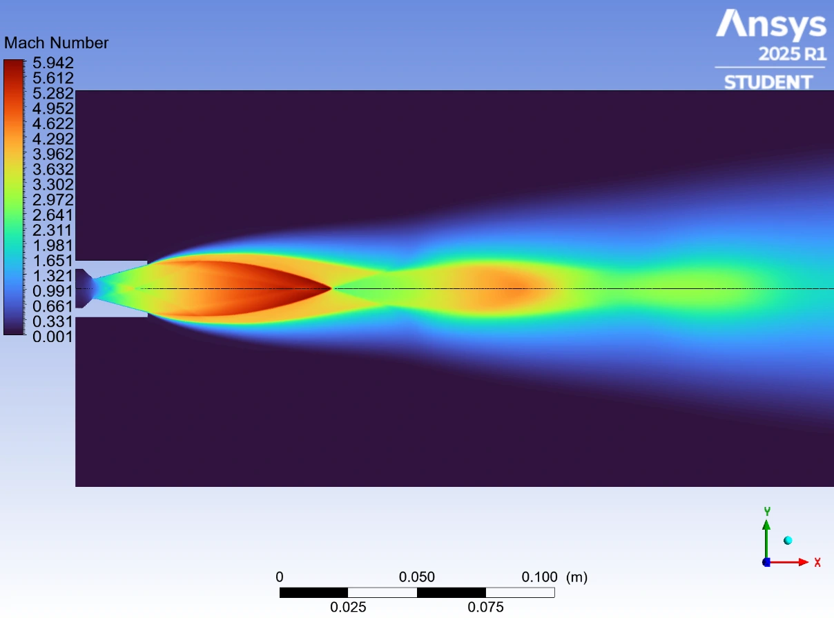
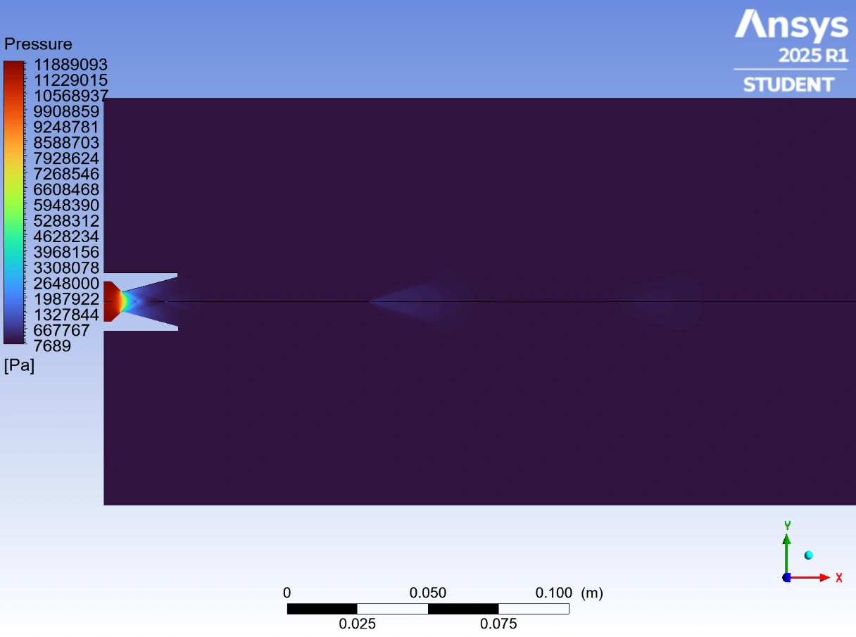
The final Mach contour shows acceleration through the converging-diverging nozzle and repeating shock structures in the external plume. Pressure decreases as the flow expands.
| Quantity | Reported value |
|---|---|
| Pressure | 212 kPa |
| Velocity | 1,770 m/s |
| Density | 0.977 kg/m³ |
| Exit area | 2.41 × 10⁻⁴ m² |
F = [ρeVe² + (Pe − Pa)]Ae
Momentum flux plus the pressure contribution at the nozzle exit.Reported CFD estimate
Calculated from the reported exit properties and nozzle area.
Reported reference peak
The estimate is approximately 9.4% below this reference value.
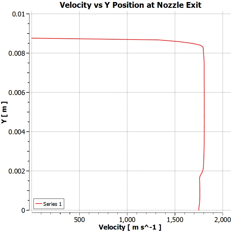
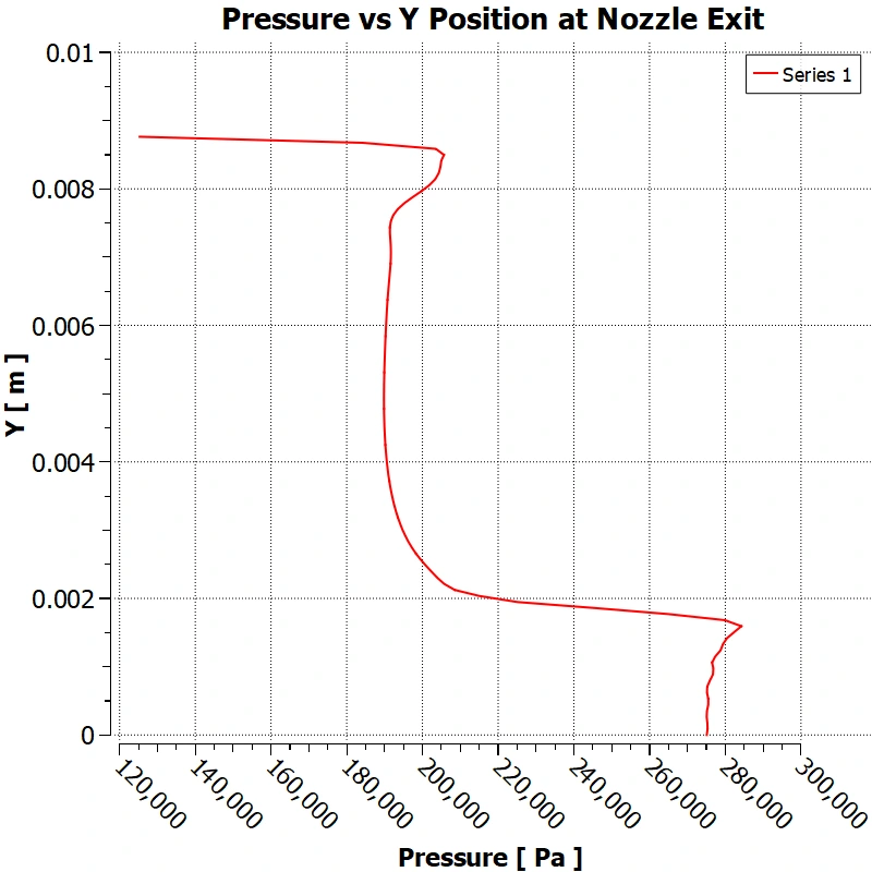
The exit profiles below show how velocity and pressure vary across the section. The calculation above uses averaged quantities, so it is an approximation to an integrated momentum-and-pressure thrust evaluation.
These are simulation results and a reference-data comparison. This project did not document a new static-fire test of the motor.
Read the original explanation · PDF p. 14 ↗07 / Lessons & next steps
The study demonstrated a practical workflow for building and improving a compressible-flow model. Its result depends on several deliberate simplifications:
The report proposes transient analysis, combustion modeling, more representative exhaust-gas properties, and three-dimensional geometry. Further verification could also include consistent convergence criteria, mass balance, and a grid study repeated with the final solver configuration.
Geometry, mesh, boundary conditions, and solver settings form one modeling system. Better results came from investigating their interaction and comparing both numerical behavior and physical flow features.
08 / Full documentation
The original 22-page PDF contains the geometry development, grid study, chamber-pressure estimates, solver configuration, results, references, and appendix plots.
All 21 embedded images are included below, including individual panels from multi-part figures. Select an image to open it at full size. Page links use PDF page numbers, which are one higher than the report’s printed numbering after the cover.

Related engineering