TUFI coating
A 2 mm modeled coating with thermal conductivity 1.5 W/(m·K). External heating reaches this surface first.
Rowan University / Heat Transfer / February 2025
Following heat.
Questioning assumptions.
An individual study of a layered spacecraft heat shield, connecting a SolidWorks drawing, thermal resistance network, analytical calculations, and a transient Simscape model.
01 / The project
How does heat move through an insulating tile and into the metal structure beneath it—and how does that structure’s temperature change with time?
My interest in thermal protection grew out of Rowan Rocketry and curiosity about reentry physics in Kerbal Space Program. For this Heat Transfer midterm project, I explored a reusable, non-ablative tile concept inspired by Starship.
I developed the annotated drawing, set up the material and boundary assumptions, formulated an energy balance, and compared analytical calculations with a Simulink / Simscape thermal model.
James Lee · Heat Transfer with Dr. Krishan Bhatia · February 25, 2025.
The TUFI coating, AETB insulation, and stainless-steel backing form the assumed material stack for this academic study. They are not presented as a verified specification of Starship’s flight hardware.
02 / Geometry & materials
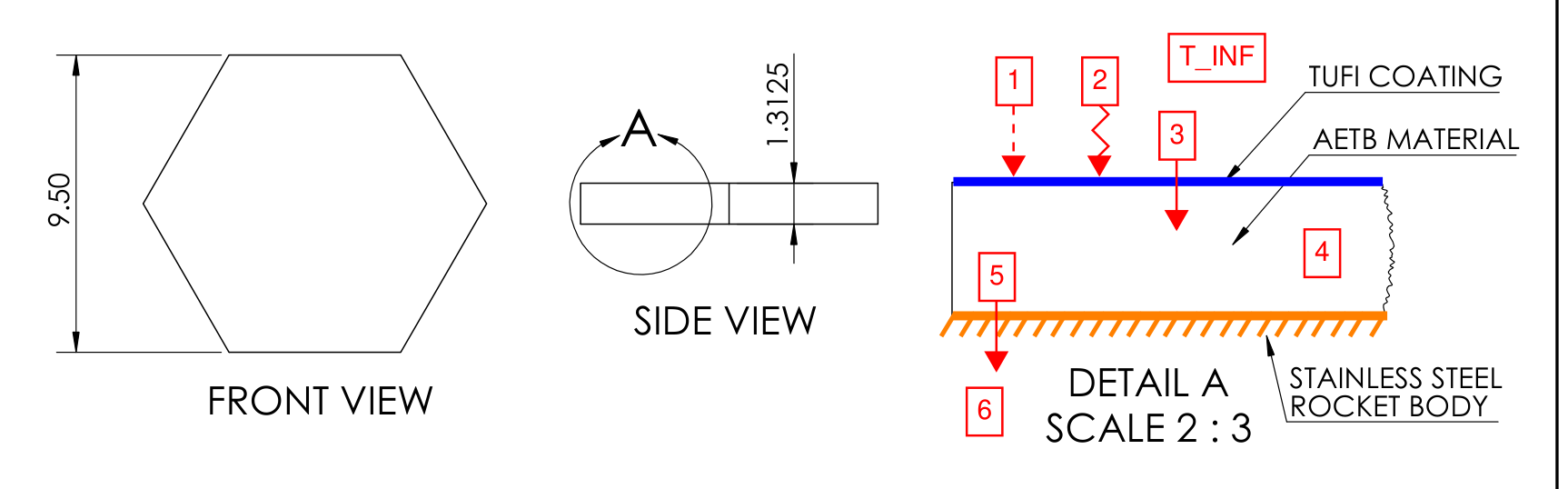
The SolidWorks drawing shows the tile’s hexagonal outline, side view, and annotated section. Its purpose is to define the modeled layers and identify convection, radiation, conduction, and thermal storage.
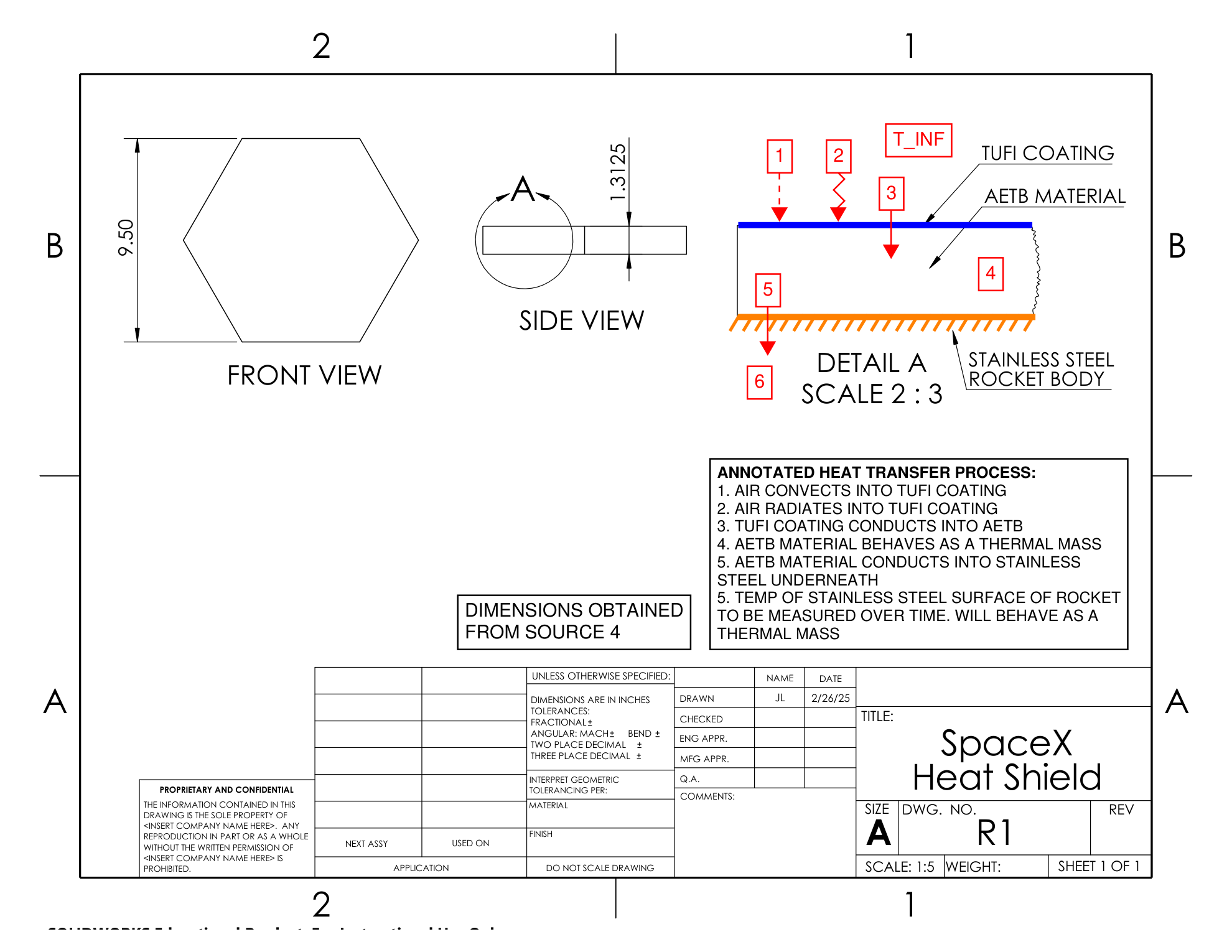
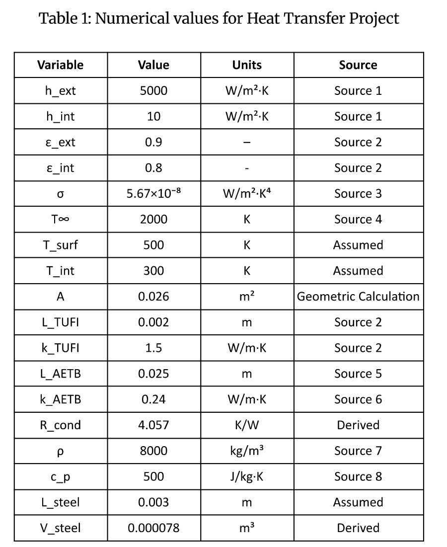
A 2 mm modeled coating with thermal conductivity 1.5 W/(m·K). External heating reaches this surface first.
A 25 mm modeled insulation layer with conductivity 0.24 W/(m·K). It supplies most of the through-thickness thermal resistance.
A 3 mm stainless-steel section with mass 0.624 kg and specific heat 500 J/(kg·K), treated as a thermal mass.
A heat-transfer area of 0.026 m² ties the layer geometry to conduction resistance and surface heat exchange.
The report combines sourced properties with assumed temperatures and dimensions. Keeping those inputs explicit makes it easier to understand which choices drive the predicted temperature.
Read the original explanation · report p. 4 ↗03 / Energy balance
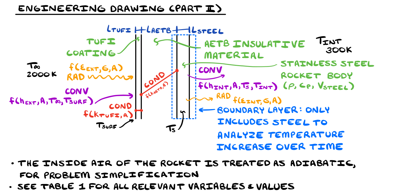
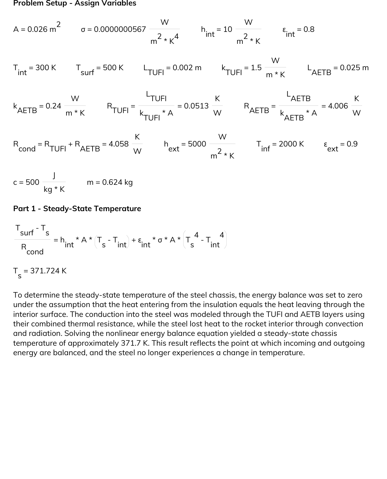
The model follows heat through the coating and insulation to the steel. On the interior side, the steel exchanges heat with a 300 K environment through convection and radiation.
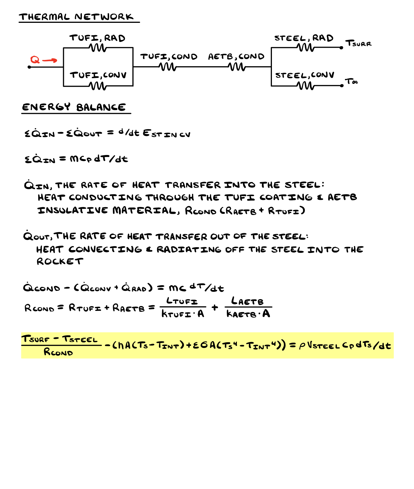
Rcond = LTUFI/(kTUFIA) + LAETB/(kAETBA)
Reported combined resistance: approximately 4.058 K/W.The insulation contributes about 4.006 K/W and the coating about 0.0513 K/W. The difference shows why the low-conductivity insulation dominates the modeled resistance.
mcpdTs/dt = Qin − Qout
Incoming conduction minus interior convection and radiation equals stored energy.The calculation includes interior heat loss. Although a handwritten note uses the word “adiabatic” for the inside air, the equations and Simscape diagram use a fixed 300 K interior boundary with convection and radiation. This page follows the implemented heat-exchange model.
Read the original explanation · report p. 5 ↗04 / Analytical model
The Blockpad calculation assumes a 500 K hot-side interface and an initial steel temperature of 300 K. It balances conduction through the two insulating layers against interior convection and radiation.
Reported equilibrium
Approximately 98.6 °C, under the analytical model’s fixed 500 K interface assumption.
Initial heating rate
At 300 K, with approximately 49.289 W entering and no initial loss to the equally warm interior boundary.
Using an interior convection coefficient of 10 W/(m²·K), a 3 mm characteristic length, and steel conductivity of 15 W/(m·K), the report calculates Bi = 0.002. This is below the usual 0.1 screening criterion for a lumped-capacitance approximation.
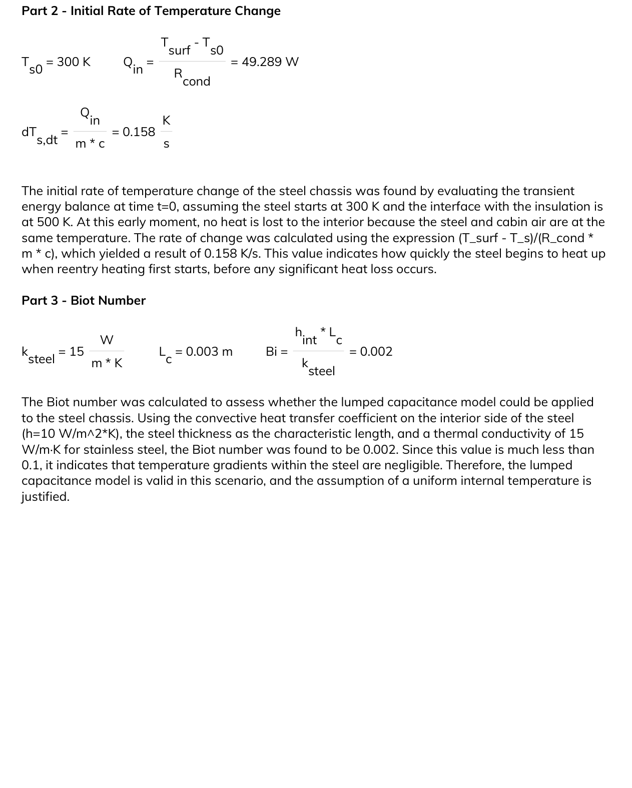
That calculation supports a uniform-temperature treatment under the selected interior convection conditions. It is a simplified check, rather than a complete assessment of every thermal boundary acting on the steel.
Read the original explanation · report p. 6 ↗05 / Transient simulation
The Simscape model starts with a 2,000 K external thermal source. It includes external convection and radiation, conduction through the TUFI and AETB layers and steel, thermal masses for insulation and steel, and interior heat exchange with a 300 K boundary.
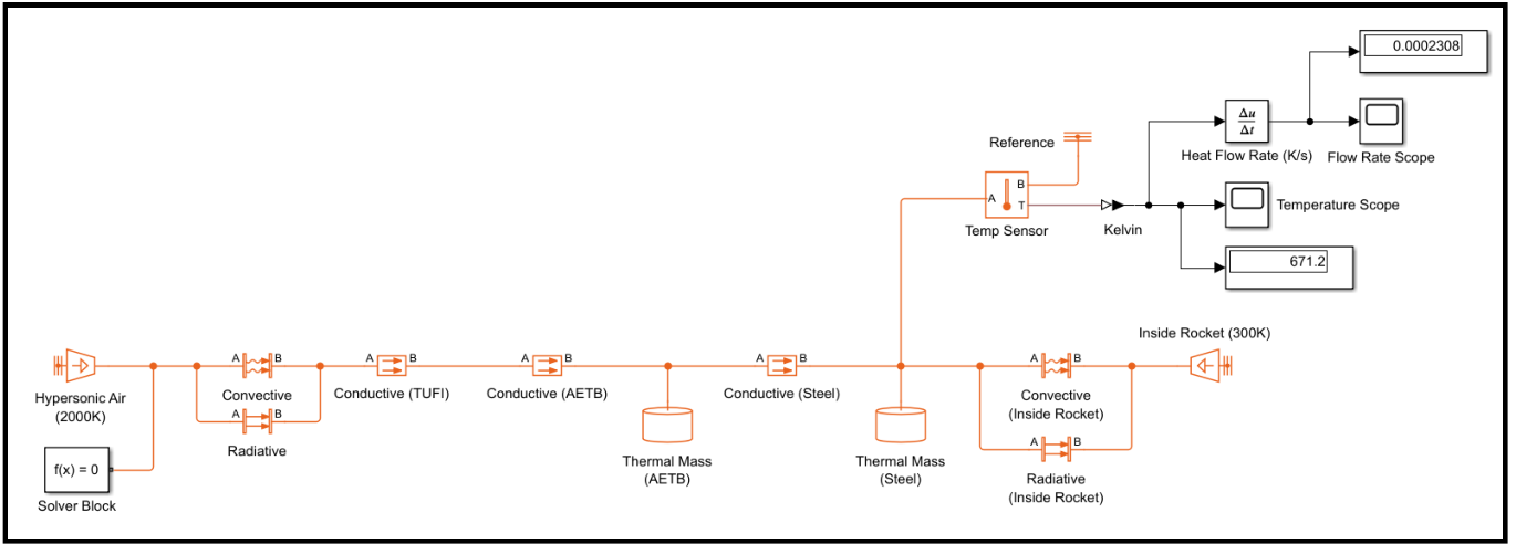
Temperature and heat-flow sensors record the steel’s response. Compared with the fixed-interface analytical calculation, the numerical model represents additional thermal storage and the path by which heat reaches the structure.
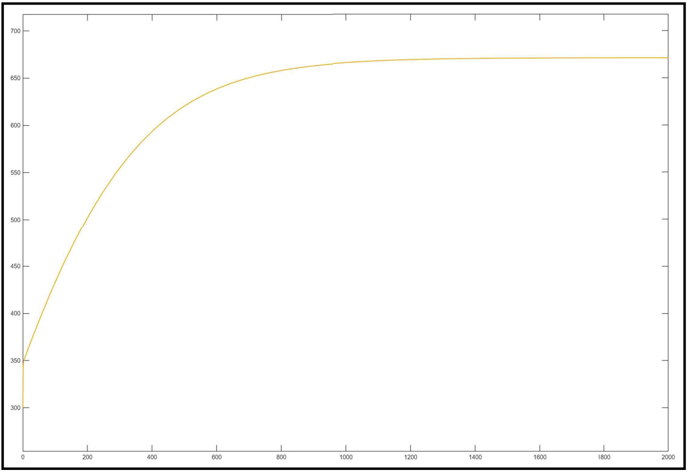
The temperature scope approaches approximately 671.2 K over the displayed simulation interval of about 2,000 seconds. This is the response to the project’s fixed conditions; it is not a flight-specific reentry trajectory or measured hardware temperature.
Read the original explanation · report p. 8 ↗06 / Comparison & lessons
The comparison is most useful as a lesson in model definition. The two calculations do not expose the steel to the same thermal boundary, so their temperature difference does not establish the accuracy of either model.
| Model | Heating boundary | Reported temperature |
|---|---|---|
| Blockpad calculation | Fixed 500 K interface | 371.7 K |
| Simscape simulation | 2,000 K external source and full layer model | 671.2 K |
The report gives a relative temperature difference of about 44.6%, using the Simscape temperature as the denominator. This describes disagreement between the models, rather than error against an experimentally established answer.
The analytical initial rate is 0.158 K/s. The report also labels the Simscape value of 0.0002308 K/s as an initial rate. That value appears in the model screenshot alongside the final temperature; the supplied record does not establish when it was sampled. An initial-rate comparison would require matching both models’ starting conditions and reading the simulation rate at time zero.
A more detailed model adds physical behavior, but its value still depends on the boundary conditions and input properties. Understanding those choices is part of understanding the result.
07 / Full documentation
The complete 10-page report includes the project motivation, annotated drawing, input table, thermal network, calculations, Simscape model, temperature response, discussion, and references.
Eight report visuals are included below. Vector drawings and handwritten pages have been rendered as images, and the simulation plots retain their original visible annotations. Select any image to open it at full size.
Related engineering