Rowan University / Fluid Mechanics / October 2024
Rocket Fins & Concrete Pumps.
Two familiar systems.
One set of fundamentals.
An individual fluid-mechanics study connecting my interests in rocketry and construction: external-flow analysis of rocket fins and an energy balance for a concrete boom pump.
- Role
- Individual course project
- External flow
- Rocket fins · 250 mph study condition
- Internal flow
- Concrete pump · 61 m boom height
- Methods
- Bernoulli · energy balance · flow simulation
01 / The project
Applying fluid mechanics to equipment I knew.
Rocket fins and concrete pumps appear unrelated, but both invite the same questions: what crosses the control volume, how energy changes, and which assumptions make the analysis useful?
Through Rowan Rocketry, I was developing a rover payload and wanted to understand more of the rocket’s aerodynamics. Through my work at Tri-State Construction, I regularly encountered concrete-pumping equipment and wanted to understand its power requirements.
For this midterm, I modeled a rocket fin, compared a simplified pressure calculation with flow-simulation results, revised the fin shape, and analyzed the pressure and power of a concrete boom pump.
Project context
James Lee · Fluid Mechanics with Dr. Krishan Bhatia · October 19, 2024.
This is an individual academic analysis inspired by my rocketry and construction experience. The report documents calculations and simulations, rather than a fabricated fin or a pump performance test.
02 / Rocket aerodynamics
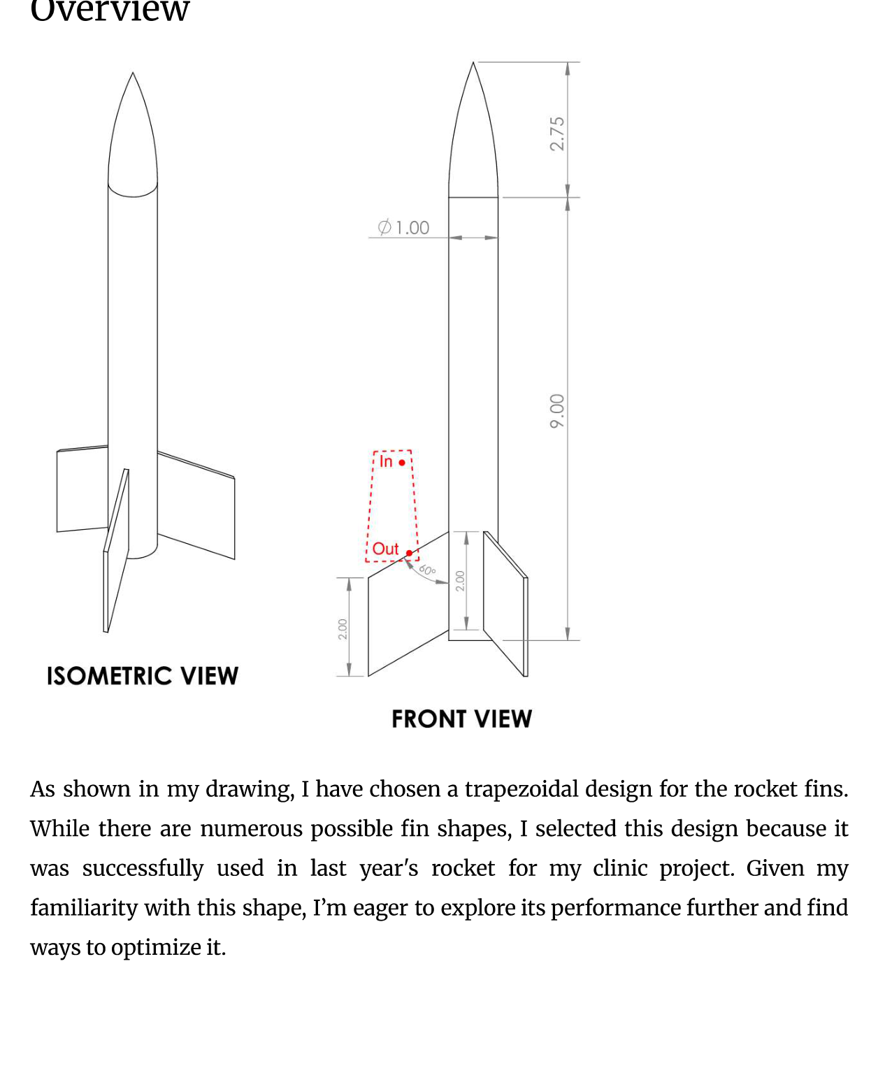
Start with a familiar trapezoidal fin.
The initial rocket drawing used trapezoidal fins, a shape familiar from our rocketry work. I selected a 250 mph study speed and treated the air as incompressible for the simplified analysis.
A first pressure and force estimate
The hand calculation used air density 1.225 kg/m³, a projected leading-face area of approximately 0.199 in², and a stagnation assumption: the local flow was treated as slowing from 250 mph to zero. The fin thickness was 0.09375 inches.
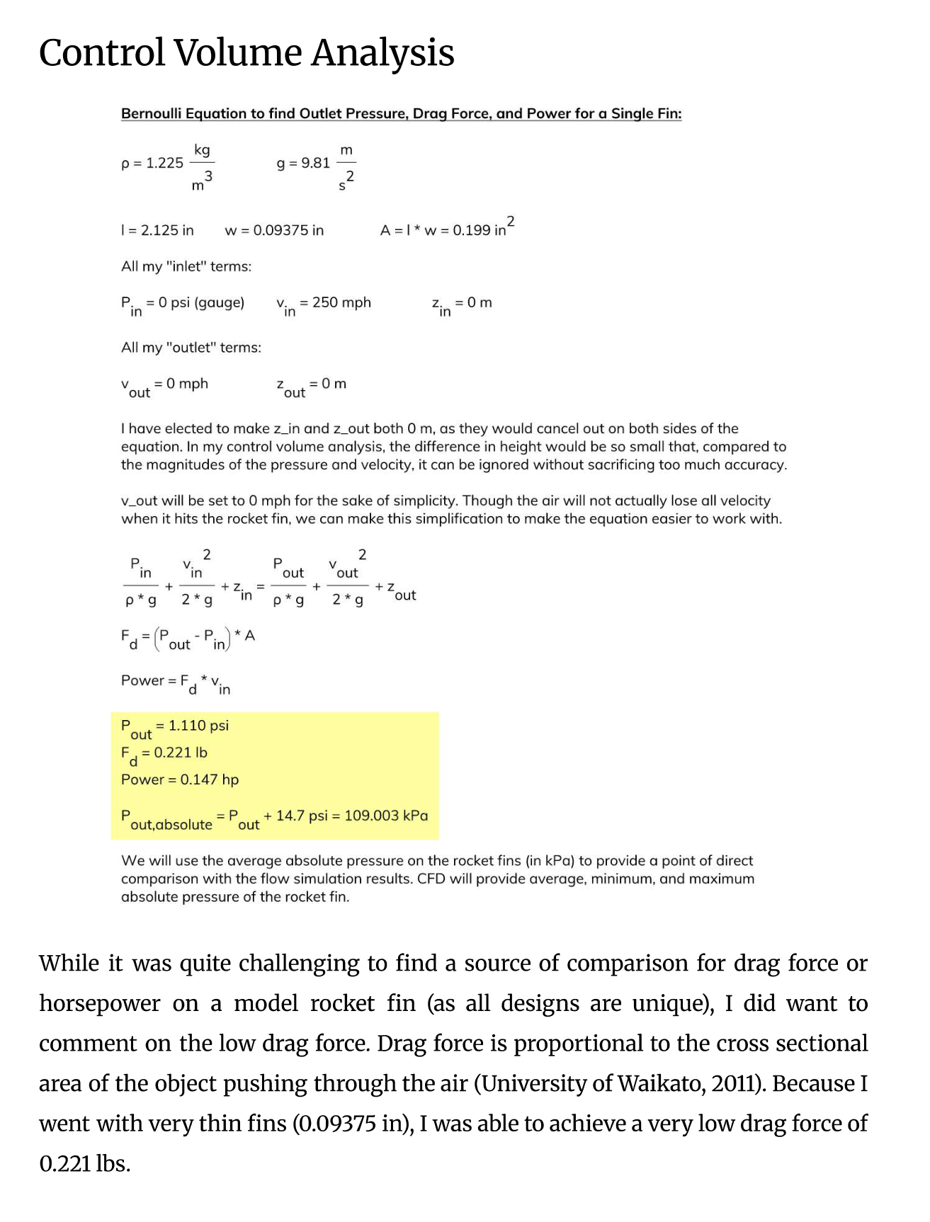
Reported pressure estimate
109.003 kPa
Absolute pressure after adding the assumed atmospheric pressure to the calculated gauge pressure.
Reported single-fin estimates
0.221 lbf · 0.147 hp
Pressure-force estimate on the projected face and its force-times-speed power equivalent.
These estimates simplify the pressure distribution and geometry. They do not represent total rocket drag or required motor power, and they omit skin friction and other aerodynamic contributions. The incompressible treatment is also an approximation at this speed.
Read the original explanation · report p. 4 ↗03 / Flow simulation
Compare the estimate with a modeled surface pressure.
The original fin’s flow simulation reported minimum, maximum, and average absolute pressures on a selected surface. Comparing the average with the hand calculation provided a way to inspect the consequences of the simplified stagnation model.
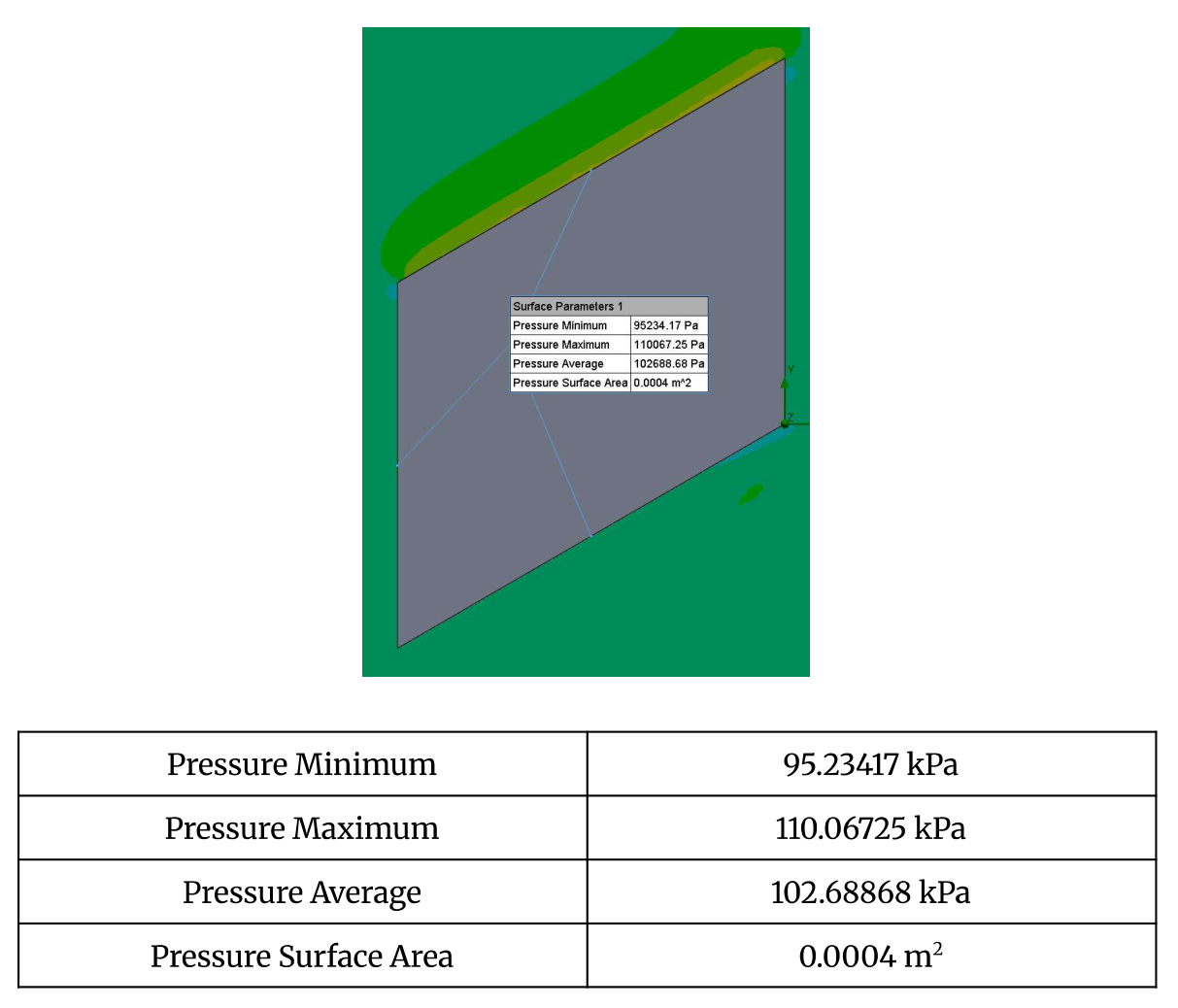
| Quantity | Value |
|---|---|
| Minimum pressure | 95.23417 kPa |
| Maximum pressure | 110.06725 kPa |
| Average pressure | 102.68868 kPa |
| Selected surface area | 0.0004 m² |
The report calculates a 5.966% difference between the 109.003 kPa analytical estimate and the 102.68868 kPa simulated average, using their mean as the denominator.
The two values describe different pressure summaries: a simplified stagnation estimate and an average over a simulated surface. Their agreement is a comparison between models, rather than a validation against measured data.
Read the original explanation · report p. 5 ↗04 / Design exploration
Replace hard edges with a rounded profile.
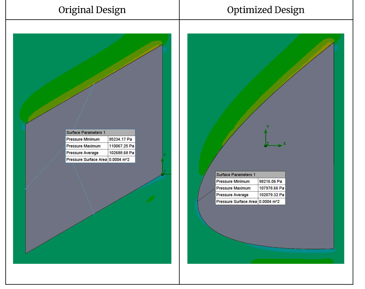
I proposed a rounded, approximately ellipsoidal fin profile while aiming to preserve the same frontal projection used in the hand calculation. The goal was to explore whether a smoother shape could reduce the modeled pressure loading.
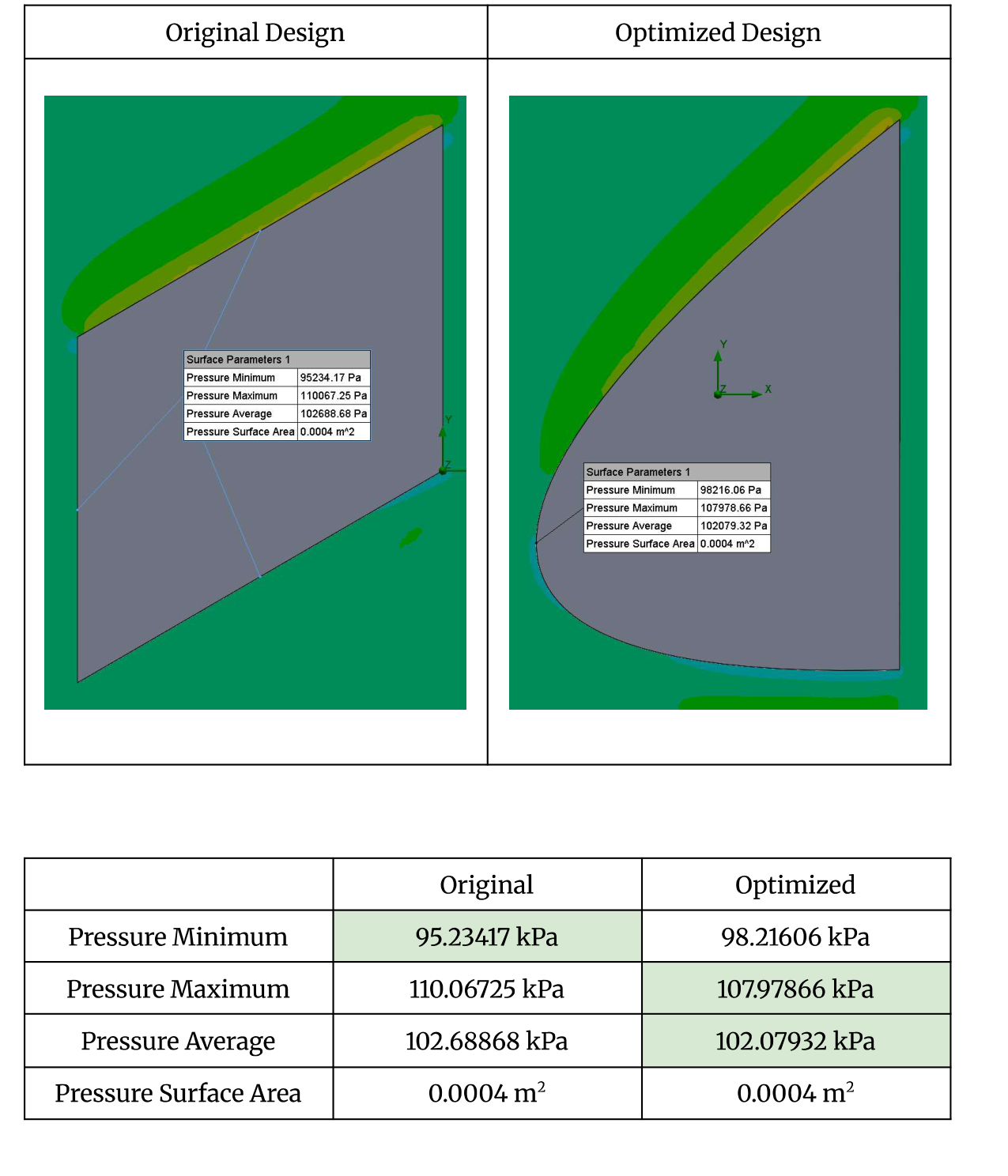
| Quantity | Original | Revised |
|---|---|---|
| Minimum pressure | 95.23417 kPa | 98.21606 kPa |
| Maximum pressure | 110.06725 kPa | 107.97866 kPa |
| Average pressure | 102.68868 kPa | 102.07932 kPa |
| Selected surface area | 0.0004 m² | 0.0004 m² |
The revised model reduced the reported average pressure by approximately 0.609 kPa and the maximum by approximately 2.089 kPa. The report describes this as an optimization; the recorded outputs establish a pressure change for the selected surface.
An integrated force calculation and drag coefficient would help establish whether this pressure change reduces total drag. Stability, structural strength, and manufacturing constraints would also matter before choosing a flight fin.
05 / Shaft work & internal flow
How much power does it take to move concrete?
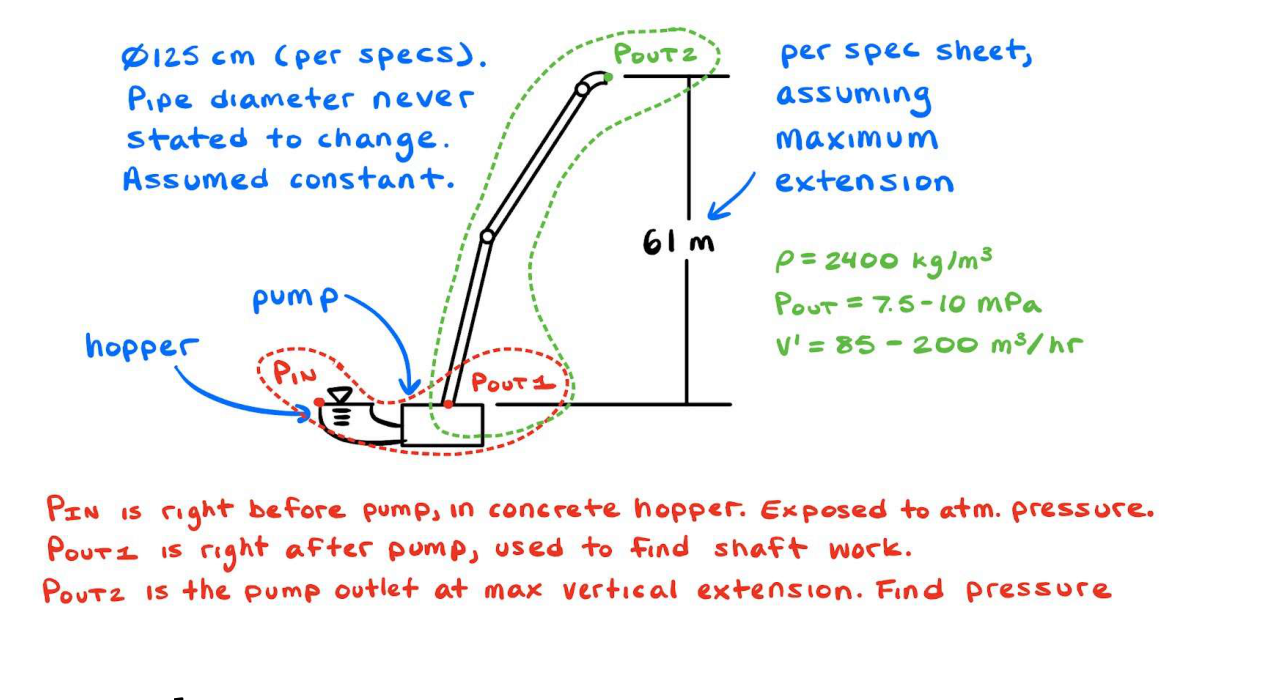
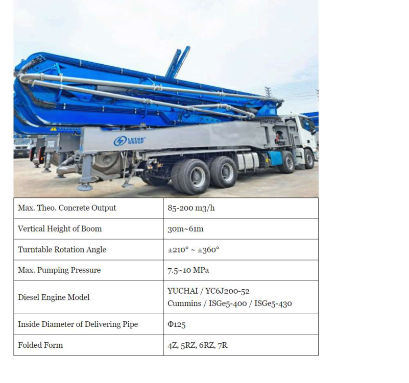
A concrete boom pump uses a powered pumping system and delivery pipe to place concrete above and away from the truck. My analysis separated the pressure rise through the pump from the elevation change along the boom.

Define the operating case
- Concrete density: 2,400 kg/m³.
- Volumetric flow: 200 m³/h, corresponding to 480,000 kg/h.
- Pump discharge: 7.5 MPa gauge.
- Maximum modeled rise: 61 m.
- Delivery pipe: 125 mm diameter, treated as constant.
An ideal pressure-rise power calculation
Phydraulic = Δp Q
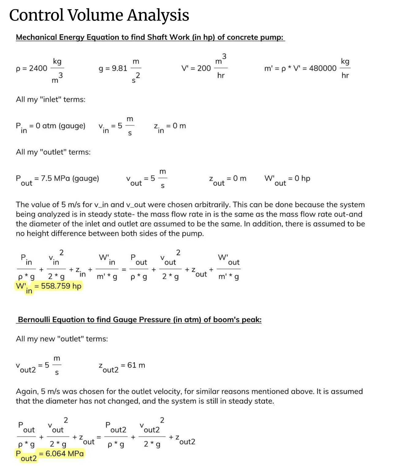
With equal inlet/outlet elevation and velocity, neglecting losses.The report’s mechanical-energy balance gives 558.759 hp, approximately 417 kW, for the selected pressure and flow. This is an ideal fluid-power requirement. Actual drive power must also account for mechanical and hydraulic efficiency and pressure losses.
Pressure at the elevated outlet
Applying Bernoulli along the boom with a 61 m rise gives a reported outlet pressure of 6.064 MPa gauge when friction losses are neglected. In that ideal model, the pressure decreases by the elevation term ρgΔz.
The outlet was not imposed as a free discharge at atmospheric pressure. The value therefore describes the assumed pressurized-flow scenario, rather than a demonstrated pressure at an open hose outlet. A practical operating-point calculation would include the discharge boundary and concrete’s flow resistance.
Read the original explanation · report p. 9 ↗06 / Interpretation & lessons
The assumptions matter as much as the arithmetic.
The report compares the calculated pump power with published Cummins engine-series ratings. The supplied comparison lists 430–605 hp, 525–565 hp, and 400–500 hp ranges.
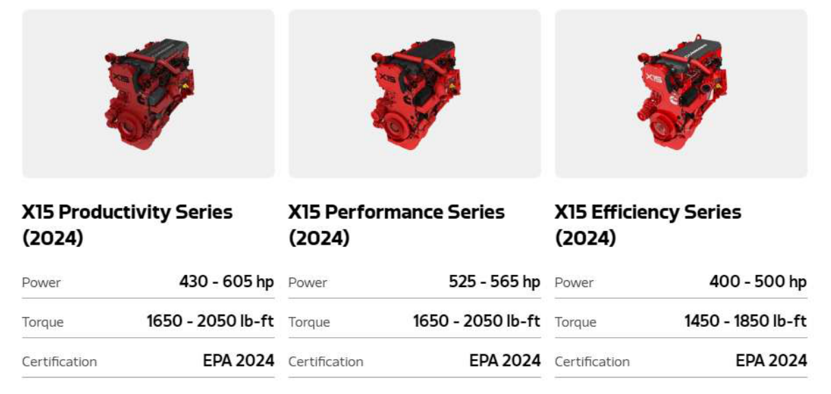
The 558.759 hp ideal requirement falls within the first two displayed ranges, but exceeds the third range’s 500 hp maximum. The source discussion says it falls within all three; the displayed specifications support the narrower comparison given here.
Even where an engine rating exceeds the ideal calculation, that alone does not prove sufficient installed capacity. Pump efficiency, accessory loads, pipe losses, and concrete’s non-Newtonian behavior affect the required power. The report identifies omitted viscous effects as an important limitation.
What the two studies taught me
- Define the control volume: a fin surface, a pump, and a delivery line require different boundaries.
- Compare the same quantity: stagnation pressure, surface-average pressure, and integrated drag are related but distinct.
- Track where energy goes: pressure rise, elevation, and losses all influence pumping requirements.
- Use specifications carefully: an engine’s rated power and ideal fluid power are different parts of the complete system.
This project brought familiar hardware into the classroom and gave me practice translating physical systems into models, comparing outputs, and identifying where a more complete analysis was needed.
07 / Full documentation
The original report and project visuals.
The complete 12-page report contains both studies, their drawings, calculations, flow-simulation results, equipment specifications, discussion, and sources.
Nine report visuals are included below. Select an image to open it at full size, or follow its page link for the original context. Equipment photographs and specification graphics are reproduced from the report and are not claimed as photographs I took.
Related engineering