Position sensing
The resistive touchscreen gives the controller an estimate of where the steel ball is on the plate.
Rowan University / Dynamic Systems and Control / 2025
Two axes.
One continuous balancing act.
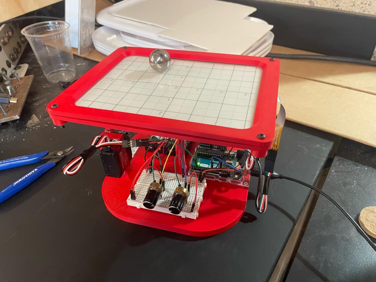
A physical feedback-control system that measures a steel ball’s position and tilts a plate to move it toward a selected target—bringing mechanical design, electronics, and PID control together.
01 / The project
Unlike a ball-and-beam system, this platform must control motion along both X and Y. A change in plate angle accelerates the ball, so reaching a target requires managing its motion as well as its position.
Our team designed and built the mechanism, integrated a resistive touchscreen and actuators, and developed a feedback controller. Two knobs set the target coordinates; the system then measures the ball’s position and continually corrects the plate tilt.
James Lee, Ian Janaszik, Zander Marks, and Vanessa Hutchinson.
Developed for Rowan University’s Dynamic Systems and Control course with Dr. Hong Zhang. This case study presents our shared engineering work.
The abstract and final results use a ±0.5-inch positioning tolerance. A separate experimental-description paragraph specifies ±0.25 inches; that inconsistency is retained in the source report and discussed alongside the results below.
Read the original explanation · report p. 2 ↗02 / Mechanical development
The team considered two- and three-servo layouts and finalized a two-servo mechanism in SolidWorks. A central universal joint supports the plate, while links from the two servos produce tilt along its axes.
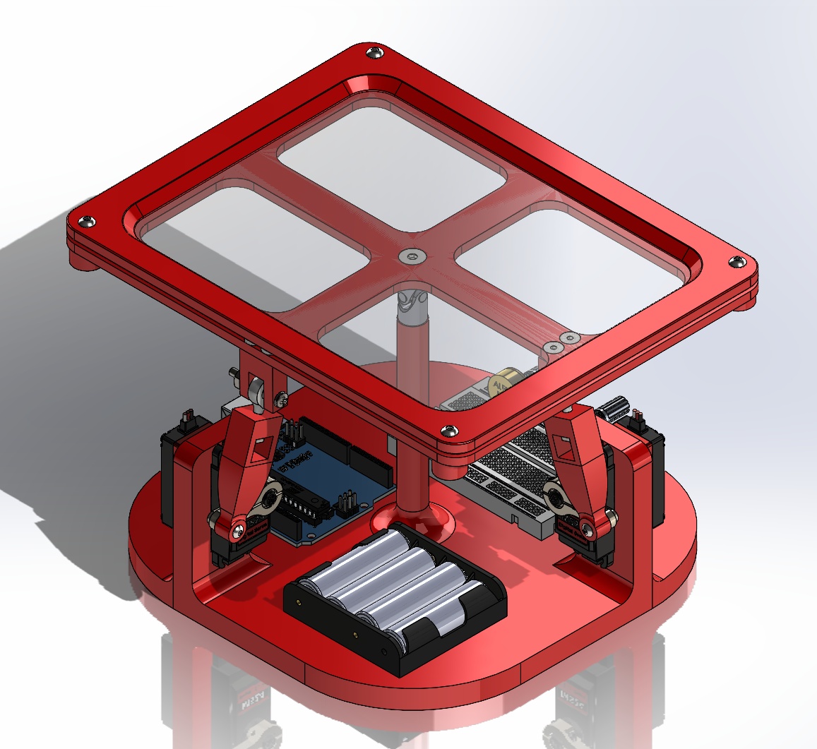
PLA parts formed the system base, servo arms, and touchscreen enclosure. The base provided mounting space for the motors, Arduino Uno, breadboard, and battery pack. Ball-joint rod ends connected the servo linkages to the plate, accommodating motion as the plate changed orientation.
The touchscreen base and top frame held the sensing surface in place. The geometry needed to maintain a usable ball surface while allowing controlled tilt and keeping the wiring accessible.
The CAD model established the actuator arrangement and available electronics space before wiring and tuning began. Packaging and control requirements influenced the mechanism together.
03 / Sensing & electronics
The Arduino Uno connected the resistive touchscreen, two B10K potentiometers, and two high-torque servo motors. The touchscreen supplied real-time position feedback; the potentiometers provided separate X and Y target inputs.
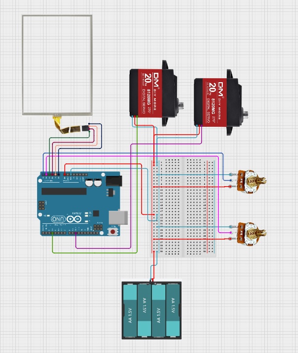
The resistive touchscreen gives the controller an estimate of where the steel ball is on the plate.
Two rotary potentiometers let the operator move the desired target without changing the program.
Two MS24 servo motors adjust the plate orientation through the printed arms and linkages.
An Arduino Uno and breadboard bring sensing, target input, and servo commands together.
The report documents four AA batteries as the power source and a shared ground between components. The schematic records the original wiring arrangement.
Read the original explanation · report p. 5 ↗04 / System dynamics
The model treats the steel ball as a uniform solid sphere rolling without slip. It neglects air resistance and uses small-angle approximations for plate tilt. These assumptions reduce the X and Y motion to matching simplified equations.
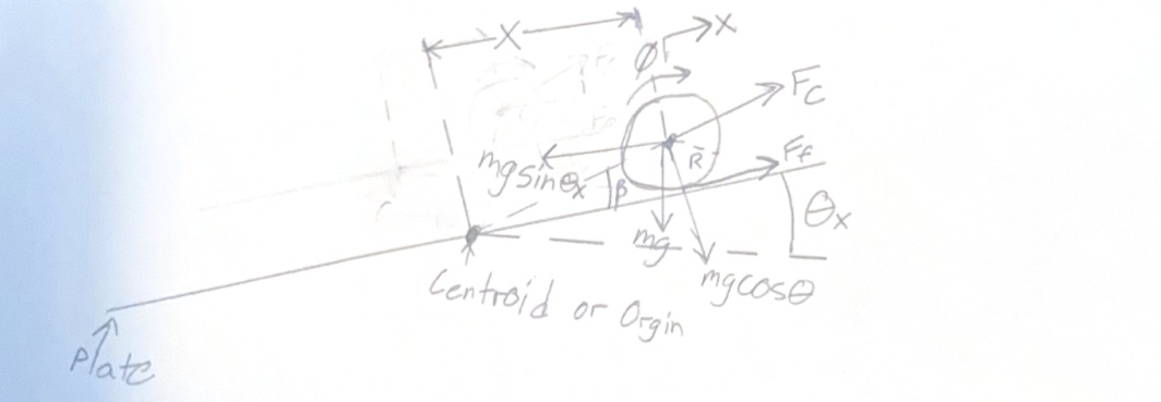
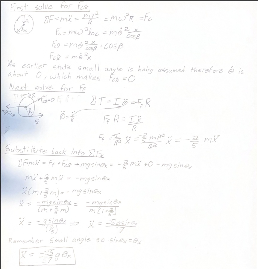
ẍ = −(5/7)gθx
ÿ = −(5/7)gθy
The angle sign follows the report’s coordinate convention.The factor 5/7 accounts for the sphere’s rotational inertia as it rolls. In Simulink, the resulting acceleration is integrated to velocity and then to position. Initial conditions represent where the ball begins.
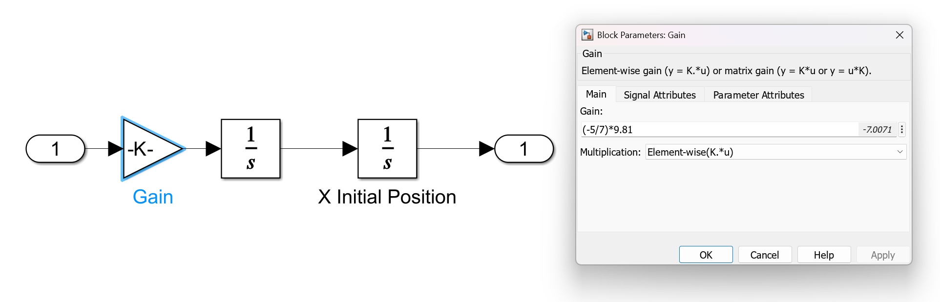
This model provides a useful control-design starting point. Linkage tolerances, sensor behavior, and effects outside the simplified assumptions still have to be addressed on the physical system.
Read the original explanation · report p. 7 ↗05 / Feedback control
The controller compares the target position with the measured position, then adjusts the servo commands to reduce that error. Separate X and Y branches use the same PID gains as a deliberate tuning simplification.
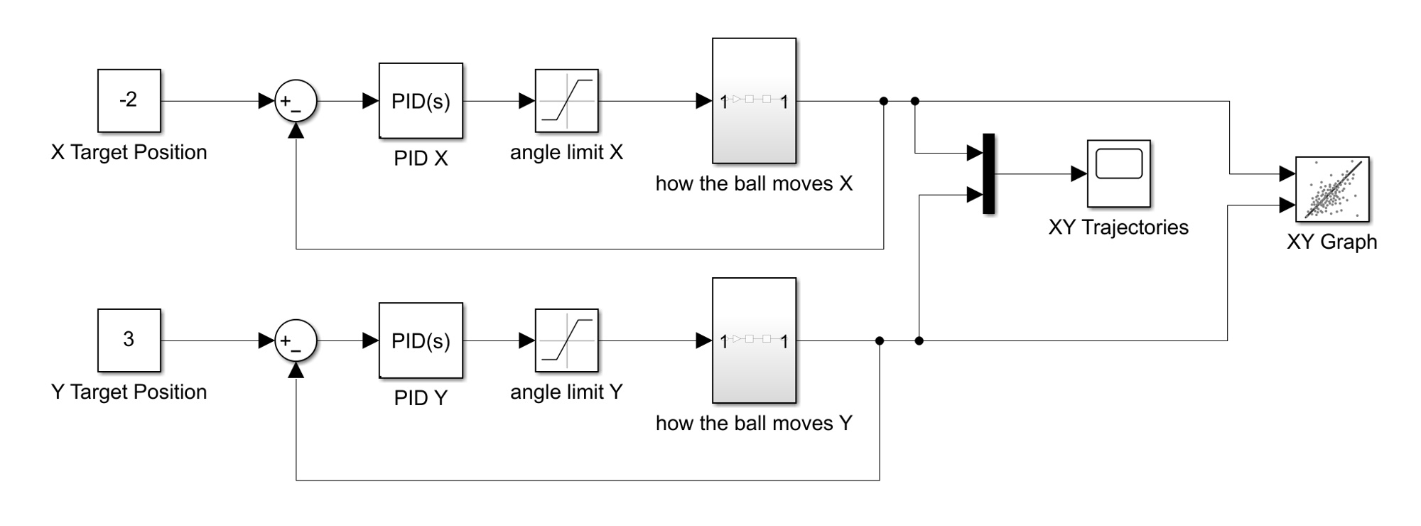
The team tuned proportional responsiveness first, then integral correction and derivative damping. The report gives the final gains as Kp = 2.5, Ki = 0.5, and Kd = 3.0, with derivative filter coefficient N = 100. These values describe this prototype and its implementation, rather than universal gains for any ball-and-plate mechanism.
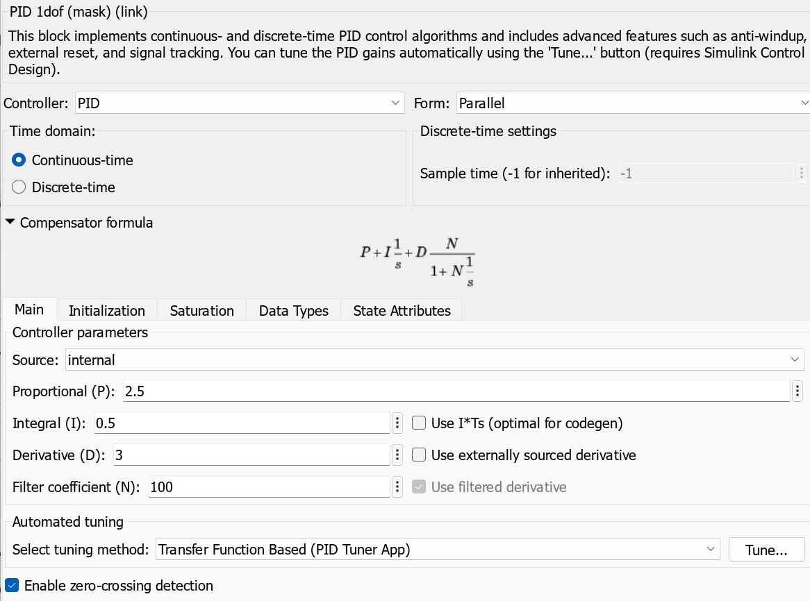
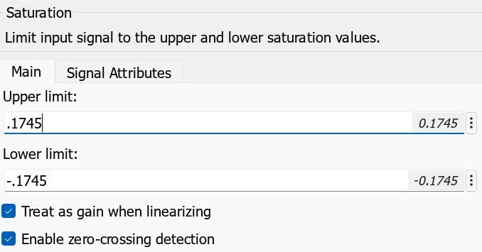
The simulation included saturation at ±0.1745 radians, approximately ±10 degrees. Limiting the tilt command represented the mechanism’s allowed motion and kept the model from demanding unrealistic actuator travel.
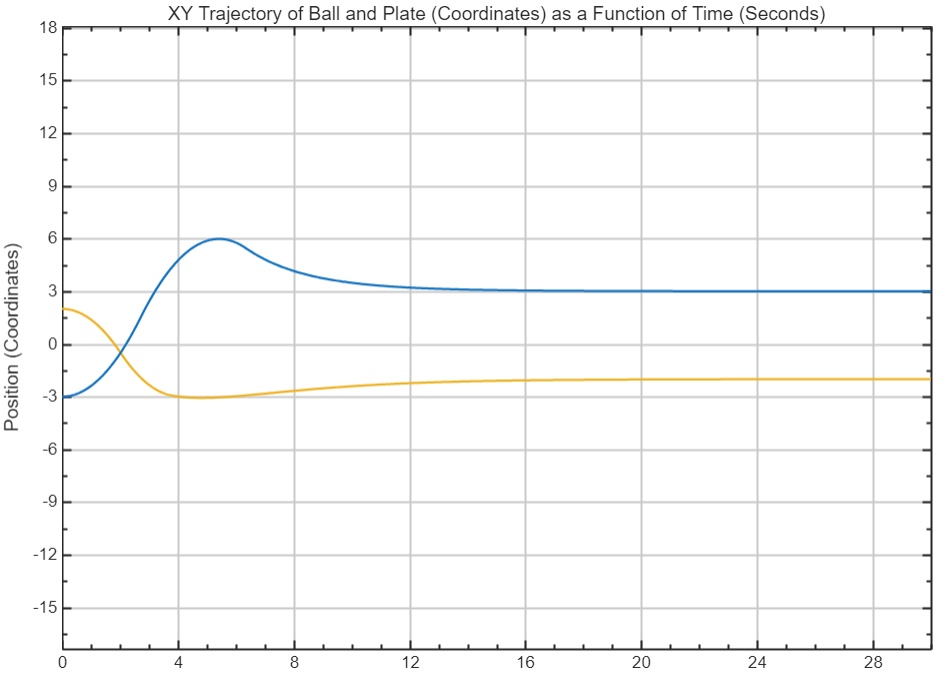
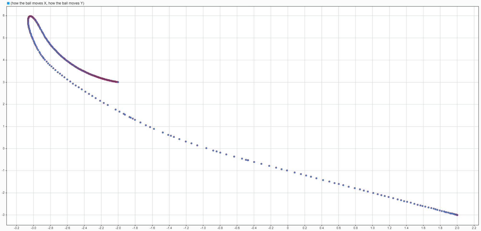
Time-history plots show the response of each axis, while the XY trajectory gives a top-down view of the modeled path. The model used the prototype’s reported gains to support comparison with the physical tuning.
06 / Testing & results
The team evaluated three target positions, timing stabilization with a stopwatch and observing recovery after manually moving the ball. The report documents 2–4-inch disturbances and 15-second steady-state holds.
Reported stabilization
Across the three recorded target tests, compared with the 20-second timing objective.
Reported recovery
Recorded recovery times after disturbances, also below the stated 20-second objective.
| Target (in) | Stabilization (s) | Disturbance (in) | Recovery (s) | Hold (s) |
|---|---|---|---|---|
| (0, 0) | 10 | 2 | 4.77 | 15 |
| (1, −1) | 5 | 4 | 8.95 | 15 |
| (−1, 1) | 5 | 3 | 7.2 | 15 |

The largest listed steady-state error component is 0.39 inches. The report concludes that the system met a ±0.5-inch tolerance, while another paragraph names a stricter ±0.25-inch requirement. Some position entries in the results table also do not match their target/error columns. The original table is shown above so those discrepancies remain visible; they have not been silently rewritten.
The reported timing results support a working stabilization and disturbance-recovery demonstration. Resolving the conflicting tolerance and coordinate entries would require the original trial records or a repeat test.
07 / Full documentation
The complete 18-page team report contains the architecture, components, dynamics derivation, Simulink model, controller tuning, and experimental results.
All 11 embedded figures are included below. Select an image to open it at full size, or follow its page link to see the original context.
Related engineering